- Monte Carlo answers a problem not by calculating it out but by playing it through randomly a thousand times over - the estimation error falls with 1/sqrt(N) and is independent of the dimension. Hence 1,000-10,000 iterations (from ~5,000 the percentile bands become smooth).
- In trading, three different things hide under 'Monte Carlo': (1) simulating price paths (GBM), (2) resampling trade sequences (robustness/drawdown), (3) permutation tests (significance/overfitting). Confusing them is the most common source of error.
- A backtest delivers ONE path of history. Monte Carlo generates the cloud of all plausible alternatives and thereby separates substance from luck. Reshuffle: same trades, different order -> same final capital, completely different drawdowns. Bootstrap (with replacement): also different final capitals, a wider cone.
- Most valuable in practice: risk of ruin and position sizing. In the illustrative example the median drawdown is 16.4%, but the 95th percentile is 27.4% and in 8.8% of runs the 25% ruin threshold is breached - all invisible in the single backtest. Industry rule of thumb: risk of ruin <= 5%.
- GBM (dS = muS dt + sigmaS dW, lognormal solution) is the standard price model, but it systematically underestimates crypto tail risk: constant vol + normal distribution ignore fat tails, vol clustering and jumps. Better choice for BTC: an empirical (block) bootstrap instead of parametric GBM.
- The critical assumption in trade reshuffling is i.i.d. (independent, identically distributed). Markets violate it through autocorrelation and regime mixing - naive shuffling UNDERESTIMATES risk of ruin. Solution: block/stationary bootstrap (Politis & Romano 1994) preserves the loss streaks.
- Permutation tests (Masters' bar permutation; White's Reality Check; Hansen SPA) are the statistically most rigorous variant against overfitting/data-snooping. This exact procedure debunked Botty's divergence hypothesis four times over (2,200 cells, only 4 with p<10% instead of ~220 expected).
- Botty already lives in the resampling family: bootstrap CIs in ml/stats.py, permutation tests in the divergence experiments, shuffle tests in the filter selection, walk-forward in ml/splits.py. The gap: no trade-sequence MC on the 3 live strategies and no risk-of-ruin-based position sizing.
- Limits: Monte Carlo does not create an edge that isn't in the data (garbage in, garbage out), does not repair lookahead/survivorship bias, does not replace out-of-sample validation and does not forecast regime changes.
What is a Monte-Carlo simulation?
A Monte-Carlo simulation answers a question not by exact calculation but by playing the problem through randomly very many times and looking at the distribution of the results. The name is an insider joke: Stanislaw Ulam, John von Neumann and Nicholas Metropolis developed the method in 1946-1948 at the Los Alamos Manhattan Project to compute neutron diffusion in an atomic bomb - a problem that was not deterministically solvable. Ulam got the idea while playing solitaire during a convalescence: instead of computing the winning probability analytically, one could simply play hundreds of games and count. Metropolis named the method after the casino in Monaco where Ulam's uncle regularly gambled away his money. The foundational paper "The Monte Carlo Method" (Metropolis & Ulam, 1949) appeared after the ENIAC had computed the first fully automatic runs.
The core in one sentence:
When a system is too complex to compute in closed form, roll the answer a thousand times over and read off the probability distribution instead of a single number.
That is exactly what makes Monte Carlo so valuable for trading: a backtest delivers exactly one path of history. But history could have unfolded differently. Monte Carlo generates the cloud of all plausible alternative paths and thereby shows how much of a backtest result was substance - and how much luck.
The mathematical foundation
Monte Carlo estimates an expected value by an average over random samples. If you want to compute E[f(X)] (e.g. the expected profit of a strategy, the option price, the ruin probability), you draw N independent samples x_1, ..., x_N from the distribution of X and form:
                  1   N
E[f(X)]  ≈  μ̂ =  ─   Σ   f(x_i)
                  N  i=1
That this works is guaranteed by the law of large numbers: mu_hat -> E[f(X)] for N -> inf. How fast it converges is stated by the central limit theorem: the estimation error is normally distributed with standard deviation
                σ_f
  Std(μ̂)  =  ─────
               √N
where sigma_f is the dispersion of f(X). Three consequences worth internalizing:
- Accuracy grows only with the square root of N. 4x as many simulations -> half the error. That is why one typically runs 1,000-10,000 iterations: below that the estimates are unstable, from ~5,000 the percentile bands become smooth.
- The error does NOT depend on the dimension of the problem. That is why Monte Carlo beats high-dimensional integrals (e.g. a portfolio of 50 correlated assets) at which classical numerical methods fail.
- From the dispersion of the simulations you get confidence intervals for free - you simply read off the 5th and 95th percentile of the result distribution.
The textbook example: estimating pi. Throw random points into a unit square with an inscribed quarter circle. The fraction of points inside the circle converges to pi/4. No one actually computes pi this way - but it shows the principle: geometry (or risk, or an option price) by rolling dice instead of by formulas.
Three families of Monte Carlo in trading
In the trading context, three methodologically different things hide under "Monte Carlo". Confusing them is the most common source of nonsense.
Family 1: Simulating price paths (Geometric Brownian Motion & co.)
Here you roll out possible futures of the price. The standard model is Geometric Brownian Motion (GBM) - the same stochastics behind Black-Scholes. The price follows the stochastic differential equation:
dS = μ S dt + σ S dW
mu is the drift (expected return), sigma the volatility, dW a Wiener process (the "random noise"). Solving this SDE with Ito's lemma yields a closed form - the price is lognormally distributed (so it can never become negative):
S_t = S_0 · exp( (μ − ½σ²) t + σ W_t )
For the simulation you discretize into small steps dt and draw a standard-normal random number Z ~ N(0,1) at each step:
S_{t+Δt} = S_t · exp( (μ − ½σ²)·Δt + σ·√Δt·Z )
Repeating this for hundreds of paths produces a fan of possible price trajectories. The following chart calibrates mu and sigma to the real BTC daily log returns 2020-2026 and simulates 400 paths over one year:
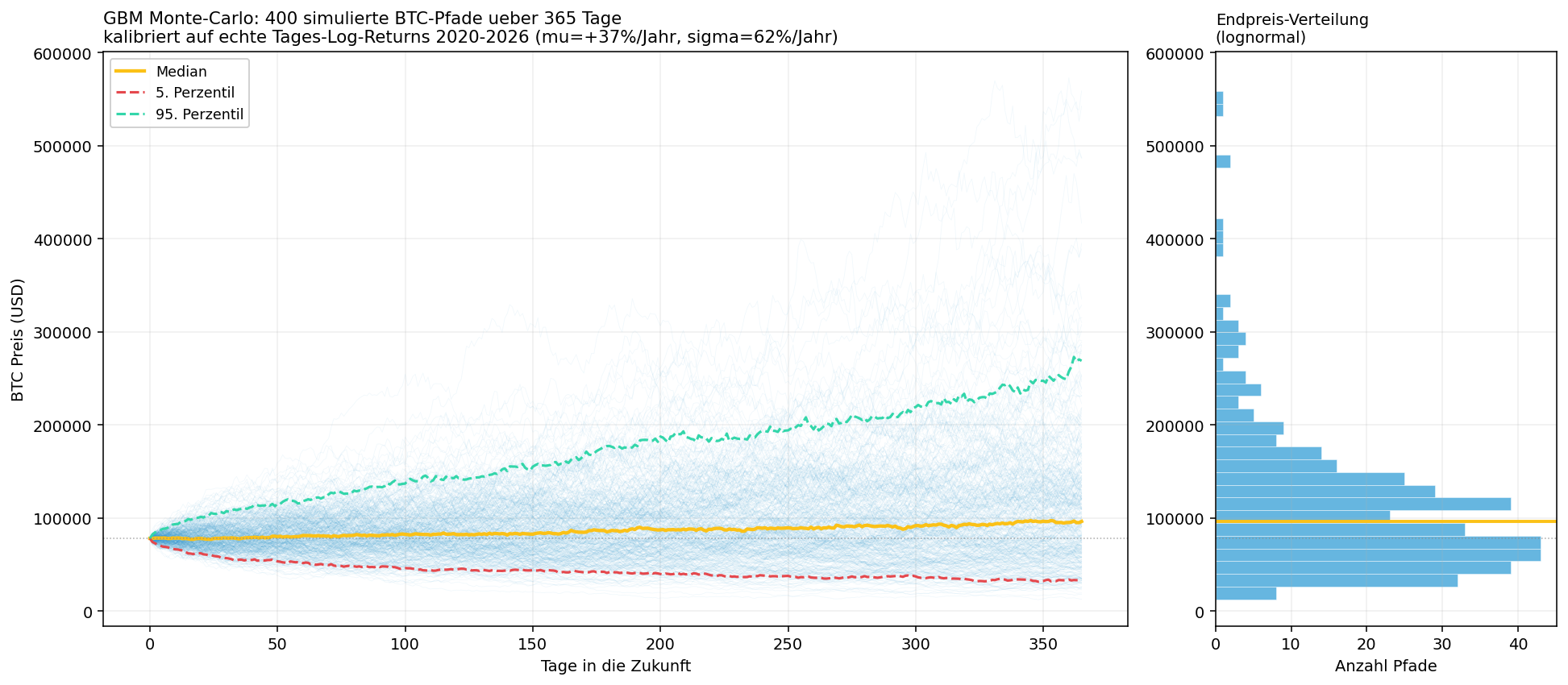
You can read off directly: from the starting price ~78,000 USD the median lands at ~96,000 USD after one year, but the 5th percentile clearly below the start, the 95th percentile a multiple above. The right-hand distribution is clearly right-skewed (lognormal) - typical for prices.
What it's used for: forward stress tests ("what does a 1-year horizon cost me in the 5% worst case?"), value-at-risk, and above all option pricing (Glasserman, Monte Carlo Methods in Financial Engineering, is the standard reference here: each path produces a final price, the option price is the discounted average of all payoffs).
Important warning for crypto: GBM assumes constant volatility and normally distributed log returns. BTC violates both drastically - fat tails (extreme moves are far more frequent than the normal distribution says), volatility clustering (calm and wild phases come in blocks) and jumps. GBM underestimates crypto tail risk systematically. Better alternatives: bootstrap of the empirical returns (no distribution model needed), block bootstrap (preserves autocorrelation, see below), GARCH models (vol clustering), jump diffusion or fractional Brownian motion (there is even an arXiv paper that models BTC with exactly that).
Family 2: Resampling trade sequences (robustness test)
This is the variant most commonly meant in trading. You take not the price but the finished trade list of a backtest and shuffle it randomly to see how fragile the pretty equity curve really is. There are three varieties (Build Alpha offers all four; the first three are the important ones):
| Method | What happens | What it shows |
|---|---|---|
| Reshuffle | Same trades, new order | Path dependence: same final capital, completely different drawdowns |
| Bootstrap (resample) | Draw trades with replacement | Wider result cone; individual trades can appear multiple times/never |
| Randomized exits | Original entries, random exits | Is the edge in the entry or is the exit overfit? |
The following chart shows reshuffle (left) vs. bootstrap (right) on an illustrative trade set (200 trades, 52% hit rate, payoff 1.5:1, 2% risk per trade, compounded multiplicatively):
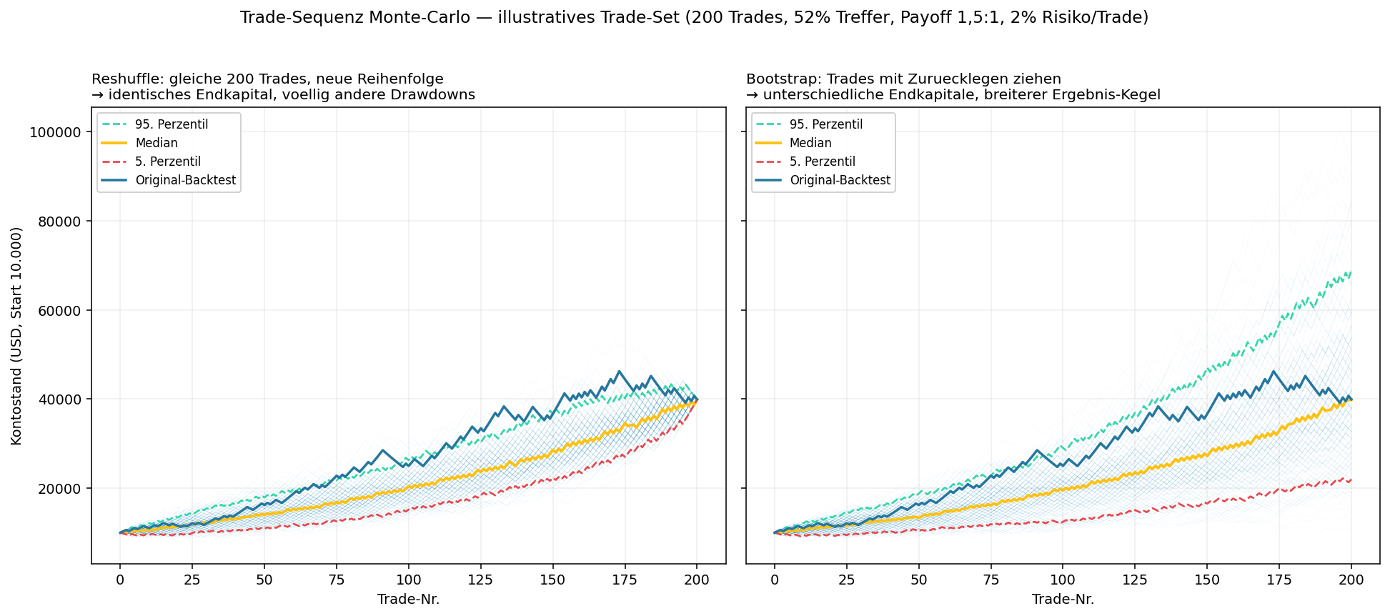
The aha moment: on the left all paths end at the same capital (same trades, just re-sorted) - but the drawdowns along the way scatter enormously. Someone who hits 12 losers in a row at the start might give up before the strategy delivers. On the right (bootstrap) the final capital also scatters widely: the 5th percentile lands at ~22,000, the 95th at ~69,000 USD - with an identical underlying edge. The single backtest path (blue line) is only one draw from this distribution.
Family 3: Permutation tests (significance & overfitting)
The statistically most rigorous variant - and the one Botty already uses. Question: Is the measured edge real or data-mining luck? You construct the null hypothesis by destroying the pattern while preserving the statistical properties:
- Label/signal permutation: Shuffle the signal timestamps randomly (Botty: 200 random masks per pattern) and see how often chance delivers an at-least-as-good mean. That fraction is the empirical p-value.
- Bar permutation (Masters): Permute the log returns between the bars and re-exponentiate to prices. This produces synthetic price data with almost identical statistical properties but destroyed patterns. If the strategy runs just as well on this fake data, its "edge" was only curve fitting. Timothy Masters' book Permutation and Randomization Tests for Trading System Development is the reference here.
- White's Reality Check / Hansen's SPA: Correct the significance when you have tested many strategies/parameters (data-snooping bias). Whoever tries 1,000 variants finds ~50 with p<5% purely by chance - these tests factor that out.
This is how Botty's divergence verdict works: across 2,200 pattern configurations only 4 delivered a p<10%, where chance would expect ~220 - worse than noise, so definitely no edge.
Risk of ruin, position sizing & drawdown distribution
The most valuable application in practice. A backtest reports one maximum drawdown. Monte Carlo (family 2) reports the entire distribution of drawdowns the same strategy could have produced:
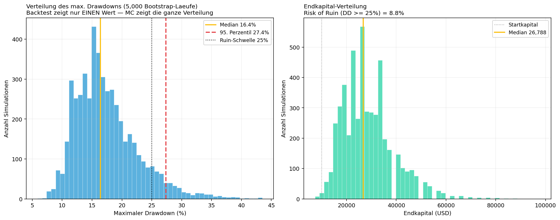
From 5,000 bootstrap runs of the same illustrative trade set: the median drawdown is 16.4%, but the 95th percentile is 27.4% - and in 8.8% of all runs the account falls below the 25% ruin threshold at some point. A single backtest that showed "only" 15% drawdown would have completely hidden this danger.
Two central concepts:
- Risk of ruin = the probability of suffering a critical capital loss (often 50%, here illustratively 25%) before the account recovers. Even strategies with a positive expected value have high ruin risk if the position size is too aggressive. Industry rule of thumb: risk of ruin <= 5% is considered acceptable.
- Position sizing from the MC drawdown analysis: You start at the 95th-percentile drawdown and work backwards to the maximum bearable risk per trade. That is more robust than sizing on the (lucky) backtest drawdown - the real worst case is, according to studies, often 2-3x the backtest drawdown.
The most important stumbling block: i.i.d. and market regime
Trade reshuffling assumes that trades are independent and identically distributed (i.i.d.). That is the central assumption - and in real markets often false:
- Autocorrelation: Losses cluster (vol clustering). Whoever shuffles trades independently smooths away exactly the loss streaks that hurt in reality -> risk of ruin is underestimated.
- Regime mixing: Mixing trades from the 2021 bull market with the 2022 bear market produces paths that could never have existed like that.
- Structural trade dependence: When one trade depends on the previous (e.g. pyramiding, trailing stops), independent shuffling is simply inadmissible.
The clean solution: the block bootstrap or stationary bootstrap (Politis & Romano, 1994). Instead of individual observations you draw contiguous blocks (with a random block length in the stationary bootstrap), so that the short-term autocorrelation is preserved. This keeps loss streaks intact and makes the risk estimate honest.
Botty's own, expensively learned lesson: A post-hoc shuffle test is invalid for strategies that re-route signals (e.g. a filter that redirects trades to a different logic). You must not shuffle the finished results - you have to re-run the complete backtest with the shuffled data source, otherwise you measure an artifact. The same family of errors as lookahead bias: the resampling must act where the causal information sits, not at the end result.
Variance reduction (for those who want it faster)
The 1/sqrt(N) convergence is slow. Instead of simply computing more paths, you can lower the dispersion sigma_f itself (Glasserman, ch. 4):
- Antithetic variates: For each path with random numbers
Z, also compute the mirror path with-Z. For (nearly) linear payoffs this eliminates almost all the variance. - Control variates: Co-simulate a correlated quantity with a known expected value and use it as a correction.
- Importance sampling: Draw from a different distribution that puts more weight on the important region (e.g. the rare tail events in risk of ruin), and re-weight with the likelihood ratio.
- Stratified / Latin hypercube sampling and quasi-Monte-Carlo (Sobol/Halton sequences instead of true randomness) distribute the samples more evenly and partly converge at
~1/Ninstead of1/sqrt(N).
Glasserman's rule of thumb: the biggest efficiency gains come from exploiting the concrete problem structure, not from generic application of these tricks.
Limits - what Monte Carlo CANNOT do
- Garbage in, garbage out. MC does not create an edge that isn't in the data - it only reshapes what is already there. If the backtest is contaminated by lookahead or survivorship, all MC runs are contaminated too.
- It does not replace out-of-sample validation. Reshuffling the same trades tests path robustness, not whether the strategy holds on unseen data. For that you need walk-forward.
- It does not forecast regime changes. A GBM calibration on the bull market says nothing about the next crash.
- Assumptions are results. Whoever assumes a normal distribution and i.i.d. gets back risk bands that are too narrow and too optimistic.
What this means for Botty
Botty already lives in the resampling family - mostly without it being called "Monte Carlo":
ml/stats.py->information_coefficient()draws 1,000 bootstrap samples for the 95% confidence interval of each IC estimate;newey_west_se()corrects for autocorrelation;downsample()reduces 1m autocorrelation before i.i.d. tests.- The divergence experiments (
ml/experiments/divergence_scan_v3/,failure_swing/) use permutation tests (200 random masks, empirical p-value) - that is family 3, textbook clean. - The filter shuffle tests (
vrp_/cvd_/bocpd_filter_shuffle_test/) and the mega-sweep filter selection build on z-scores from shuffled runs. - Walk-forward + purged CV (
ml/splits.py) is the complementary out-of-sample discipline.
The gap: On the three live strategies there is so far no classical trade-sequence Monte-Carlo (family 2). We know exactly one backtest drawdown per strategy - not the distribution. And the position sizing (execution/config.py: POSITION_SIZE_PCT, MAX_POSITION_USD) is not derived from a risk-of-ruin analysis. This is exactly where the next concrete step lies (see recommendations).
Code & to reproduce
- Chart generator for this article:
research/recherchen/assets/_gen_montecarlo_chart.py - Botty's bootstrap CIs:
ml/stats.py(information_coefficient,newey_west_se) - Botty's permutation test:
ml/experiments/divergence_scan_v3/run.py