Data Overview
entryBTCUSDT — Data Overview
🎯 Mai-2026-Welle ABGESCHLOSSEN: Roadmap · Synthesis-Report — 9 Experimente, 4 promoted (BOCPD, ETF-Flow, DVOL/VRP, Master-LGBM, R²+10.6pp), 2 pursue, 3 dropped.
Generated by ml/overview.py on 2026-05-17 09:32 UTC. Source: Binance USDM 1m futures via backtesting/data/.
This report is the entry point for the ml/ pattern-discovery module. It is descriptive, not prescriptive — every conditional edge spotted here must be re-validated walk-forward in ml/experiments/ before feeding a strategy.
1. Data coverage
- Range: 2020-01-01T00:00:00+00:00 → 2026-04-28T23:59:00+00:00 (2,309 days, 6.3 years)
- Bars: 3,326,400 (expected 3,326,400, completeness 100.000%)
- Gaps > 60s: 0 (max gap 60s)
- Zero-volume bars: 369 (0.0111%)
- Price range: $3,707 → $126,087
- Funding: 2023-05-12 → 2026-05-13 (25,773 settlements)
Per-year coverage
| timestamp | bars | zero_vol_bars | first | last | close_lo | close_hi |
|---|---|---|---|---|---|---|
| 2020 | 527040 | 2 | 2020-01-01 | 2020-12-31 | 3706.96 | 29336 |
| 2021 | 525600 | 59 | 2021-01-01 | 2021-12-31 | 28180 | 69154.9 |
| 2022 | 525600 | 64 | 2022-01-01 | 2022-12-31 | 15502 | 48143 |
| 2023 | 525600 | 118 | 2023-01-01 | 2023-12-31 | 16497.1 | 44745 |
| 2024 | 527040 | 89 | 2024-01-01 | 2024-12-31 | 38560.6 | 108225 |
| 2025 | 525600 | 37 | 2025-01-01 | 2025-12-31 | 74585.8 | 126087 |
| 2026 | 169920 | 0 | 2026-01-01 | 2026-04-28 | 60003.9 | 97794.3 |
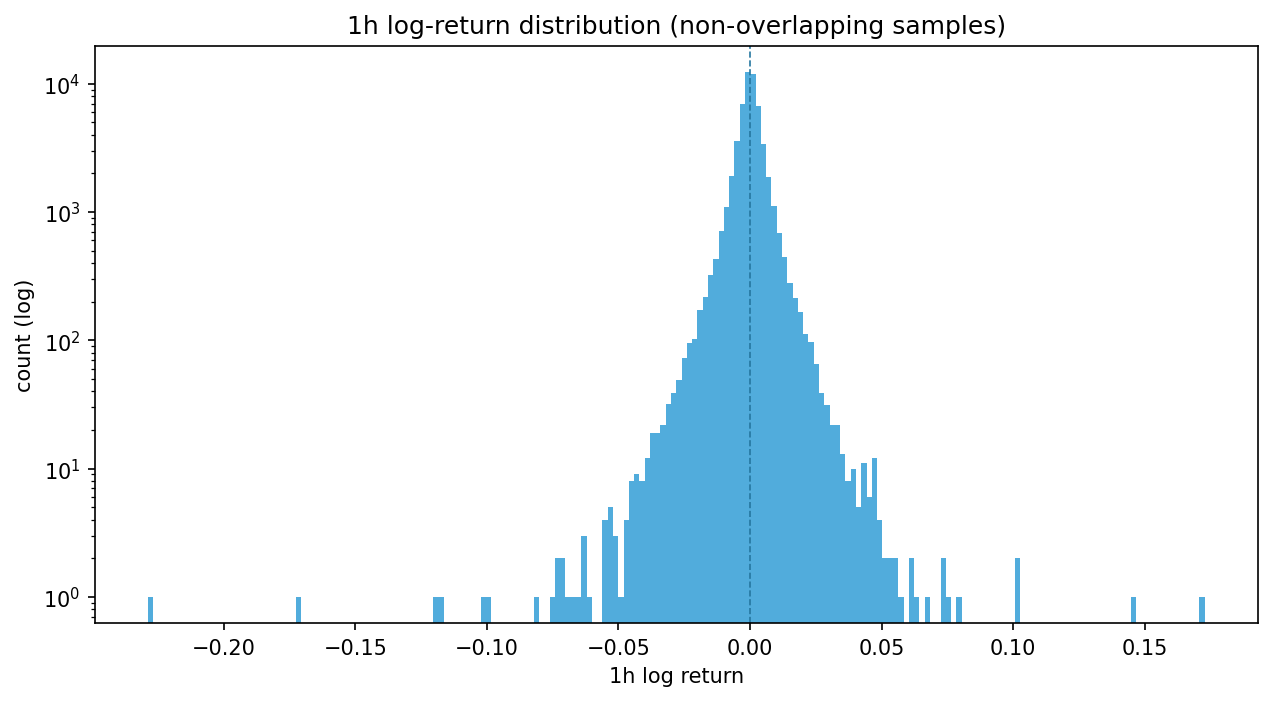
2. Return distributions across horizons
Log returns at multiple horizons. Vol_annual is the per-bar std scaled by sqrt(periods_per_year). High excess kurtosis indicates fat tails; positive skew means more positive shocks than negative.
| horizon | n_obs | mean | std | vol_annual | skew | kurt_excess | p01 | p05 | p50 | p95 | p99 | tail_3sigma_pct |
|---|---|---|---|---|---|---|---|---|---|---|---|---|
| 1m | 3,326,399 | 0 | 0.0009 | 0.6741 | -0.2411 | 193.04 | -0.0025 | -0.0012 | 0 | 0.0012 | 0.0025 | 1.4976 |
| 5m | 665,279 | 0 | 0.002 | 0.6579 | -1.0969 | 140.5 | -0.0056 | -0.0026 | 0 | 0.0026 | 0.0056 | 1.6115 |
| 15m | 221,759 | 0 | 0.0034 | 0.6451 | -0.3687 | 92.5615 | -0.0097 | -0.0045 | 0 | 0.0045 | 0.0096 | 1.6784 |
| 1h | 55,439 | 0 | 0.0067 | 0.6274 | -0.8929 | 63.0225 | -0.0196 | -0.0091 | 0.0001 | 0.0091 | 0.0191 | 1.7966 |
| 4h | 13,859 | 0.0002 | 0.0131 | 0.6113 | -0.7419 | 18.2072 | -0.0392 | -0.0193 | 0.0002 | 0.0193 | 0.038 | 1.9193 |
| 1d | 2,309 | 0.001 | 0.0326 | 0.6229 | -1.4664 | 24.825 | -0.088 | -0.0481 | 0.0005 | 0.05 | 0.0923 | 1.5158 |
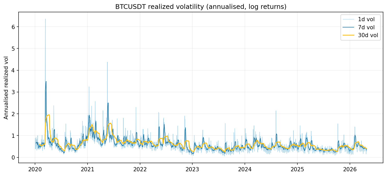
3. Volatility regimes over time
Annualised realized vol from 1m close-to-close returns, rolling over different windows. Look for regime breaks and clustering.
Annualised vol per year
| timestamp | ann_vol_1d_avg | ann_vol_1d_min | ann_vol_1d_max | biggest_1d_move_pct |
|---|---|---|---|---|
| 2020 | 0.642 | 0.116 | 7.254 | 72.185 |
| 2021 | 0.869 | 0.38 | 4.521 | 38.705 |
| 2022 | 0.595 | 0.076 | 2.467 | 21.653 |
| 2023 | 0.402 | 0.049 | 1.593 | 18.62 |
| 2024 | 0.511 | 0.106 | 2.142 | 20.889 |
| 2025 | 0.418 | 0.086 | 1.594 | 15.936 |
| 2026 | 0.486 | 0.103 | 1.637 | 19.467 |
4. Autocorrelation: returns vs |returns|
Returns themselves should have near-zero autocorrelation (efficient market). |returns| typically show strong positive autocorrelation (volatility clustering). The gap between them is the signature of GARCH-style dynamics.
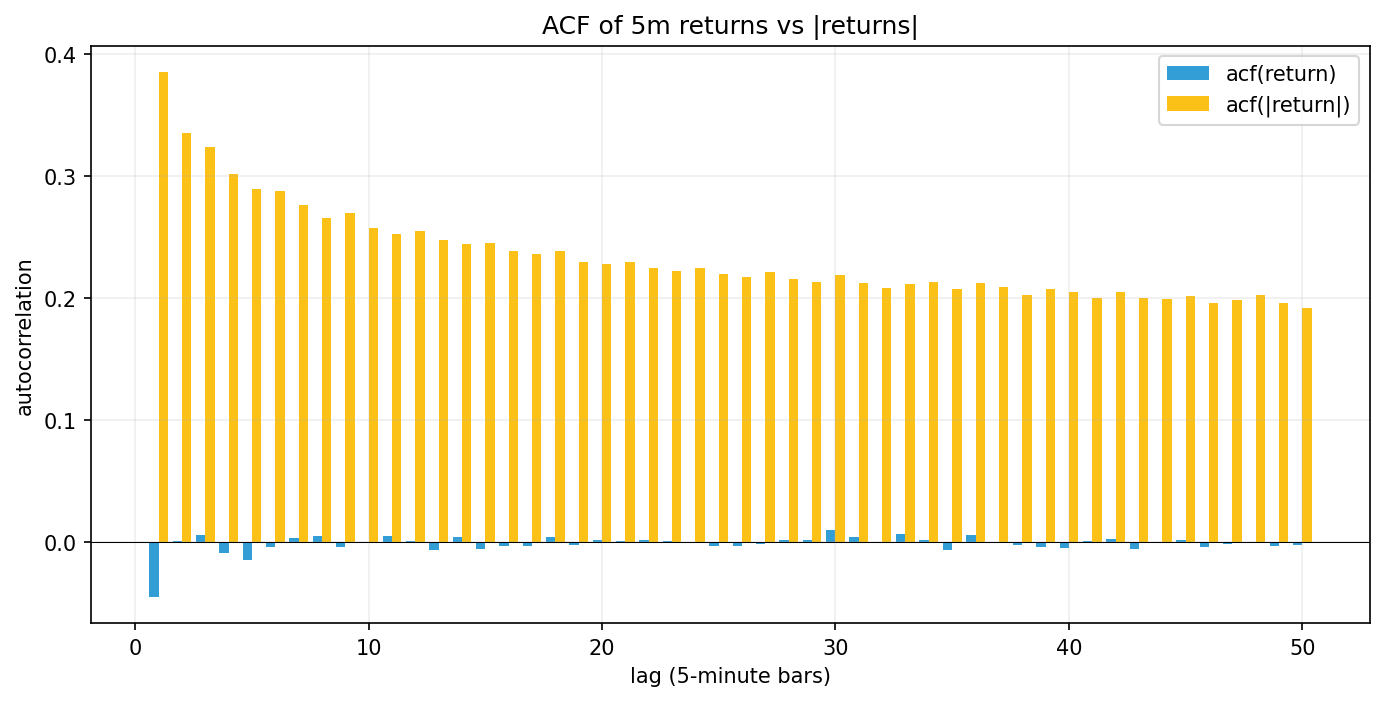
- Lag-1 acf(return) = -0.0453 (mean-reversion)
- Lag-1 acf(|return|) = +0.3851 (strong vol clustering if > 0.1)
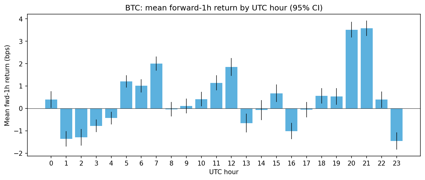
5. Time-of-day & day-of-week effects
Mean and std of forward 1h log returns grouped by UTC hour and by weekday. t-stat = mean / (std / sqrt(n)) — rough significance check.
⚠️ Caveat: consecutive 1m bars produce overlapping 60-bar forward windows, so observations within the same hour are heavily correlated. The reported
noverstates the effective sample size by roughly 60×, which inflates t-stats. Treat large t-stats as a screening signal — confirm walk-forward inml/experiments/with non-overlapping samples before believing.
By UTC hour
| hour | mean_bps | std | count | t_stat |
|---|---|---|---|---|
| 0 | 0.4 | 0.00701 | 138600 | 2.1 |
| 1 | -1.36 | 0.00659 | 138600 | -7.68 |
| 2 | -1.29 | 0.00709 | 138600 | -6.77 |
| 3 | -0.78 | 0.00539 | 138600 | -5.39 |
| 4 | -0.43 | 0.00532 | 138600 | -3.02 |
| 5 | 1.21 | 0.00519 | 138600 | 8.65 |
| 6 | 1.01 | 0.00556 | 138600 | 6.77 |
| 7 | 2 | 0.00588 | 138600 | 12.68 |
| 8 | -0.04 | 0.00611 | 138600 | -0.24 |
| 9 | 0.11 | 0.0063 | 138600 | 0.64 |
| 10 | 0.41 | 0.00612 | 138600 | 2.51 |
| 11 | 1.14 | 0.00641 | 138600 | 6.65 |
| 12 | 1.85 | 0.00745 | 138600 | 9.25 |
| 13 | -0.65 | 0.00807 | 138600 | -3.02 |
| 14 | -0.08 | 0.00854 | 138600 | -0.33 |
| 15 | 0.68 | 0.00748 | 138600 | 3.36 |
| 16 | -1.01 | 0.00685 | 138600 | -5.51 |
| 17 | -0.06 | 0.00646 | 138600 | -0.34 |
| 18 | 0.56 | 0.0065 | 138600 | 3.2 |
| 19 | 0.54 | 0.00699 | 138600 | 2.85 |
| 20 | 3.51 | 0.00667 | 138600 | 19.6 |
| 21 | 3.58 | 0.00647 | 138600 | 20.61 |
| 22 | 0.39 | 0.00691 | 138600 | 2.11 |
| 23 | -1.46 | 0.00731 | 138540 | -7.42 |
By day-of-week (Mon-Sun)
| mean_bps | std | count | t_stat | |
|---|---|---|---|---|
| Mon | 1.62 | 0.00733 | 475200 | 15.25 |
| Tue | 0.24 | 0.00666 | 475140 | 2.48 |
| Wed | 2.05 | 0.00707 | 475200 | 20 |
| Thu | -1.55 | 0.00724 | 475200 | -14.78 |
| Fri | 0.51 | 0.00743 | 475200 | 4.71 |
| Sat | -0.03 | 0.0049 | 475200 | -0.45 |
| Sun | 0.15 | 0.00556 | 475200 | 1.83 |
6. Volume & activity patterns
Where does the action concentrate? Volume rhythms hint at when liquidity providers vs. takers dominate. Also a sanity check for time-of-day return effects.
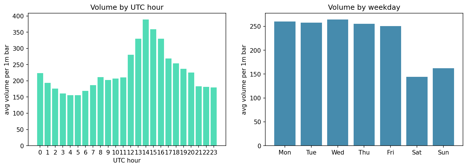
Avg volume per 1m bar by UTC hour
| timestamp | avg_vol |
|---|---|
| 0 | 223.77 |
| 1 | 193.69 |
| 2 | 176.29 |
| 3 | 160.65 |
| 4 | 155.61 |
| 5 | 155.74 |
| 6 | 168.51 |
| 7 | 186.4 |
| 8 | 211.37 |
| 9 | 202.09 |
| 10 | 207.19 |
| 11 | 210.28 |
| 12 | 280.38 |
| 13 | 329.89 |
| 14 | 389 |
| 15 | 359.16 |
| 16 | 330.08 |
| 17 | 268.79 |
| 18 | 253.77 |
| 19 | 237.39 |
| 20 | 225.27 |
| 21 | 182.8 |
| 22 | 181.35 |
| 23 | 179.59 |
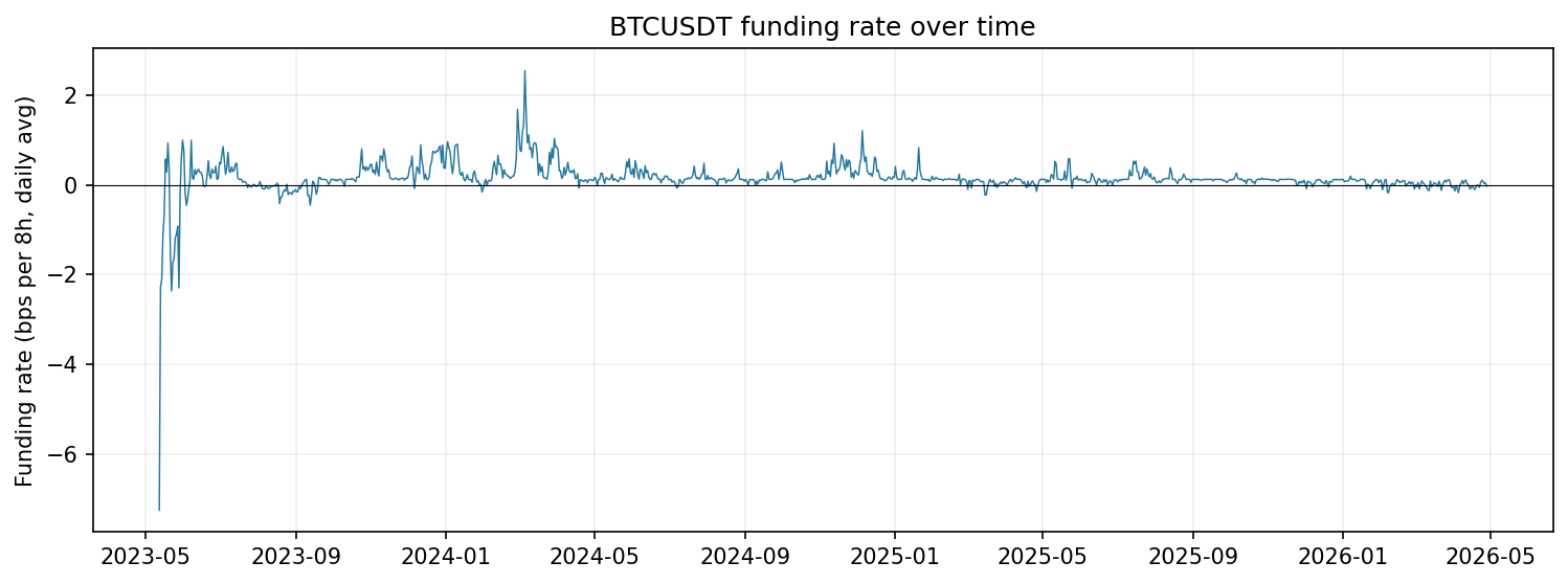
7. Funding rate analysis
- Coverage: 2023-05-12 → 2026-04-28 (1,559,519 bars with funding attached)
- Mean per 8h: +0.153 bps
- Std per 8h: 0.417 bps
- Annualised (×1095): mean 1.68% / std 4.56%
- Min / Max single settlement: -8.18 bps / +5.98 bps
- % bars with negative funding: 13.81%
Forward-24h return by funding quintile (sampled at 8h settlements)
Quintiles use rank-based ties when funding-rate buckets collide on the default value. |t-stat| > 2 suggests the bucket's mean is unlikely zero — but settlements 24h apart can overlap, so treat as a hint not proof.
| mean_bps | std | count | t_stat | |
|---|---|---|---|---|
| Q1 (-0.0018180000000000002, 5.86e-06] | 29.8 | 0.021 | 649 | 3.62 |
| Q2 (5.86e-06, 1.25e-05] | -3.1 | 0.0238 | 1809 | -0.56 |
| Q3 (1.25e-05, 2.41e-05] | -16.2 | 0.0248 | 138 | -0.77 |
| Q4 (2.41e-05, 0.000453] | 31.5 | 0.0249 | 649 | 3.22 |
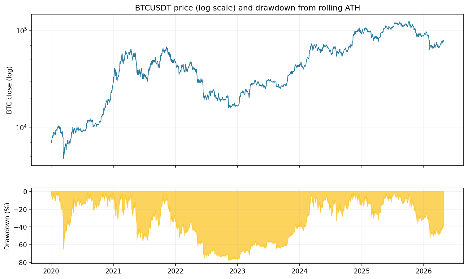
8. Bull / bear regimes & drawdowns
Top-10 drawdown episodes (peak-to-trough within sample)
| start | end | length_days | max_dd_pct | peak_price | trough_price |
|---|---|---|---|---|---|
| 2021-11-10 | 2024-03-08 | 849 | -77.6% | $69,155 | $15,502 |
| 2020-02-13 | 2020-07-27 | 165 | -64.8% | $10,535 | $3,707 |
| 2021-04-14 | 2021-10-20 | 189 | -55.6% | $64,945 | $28,860 |
| 2025-10-06 | 2026-04-28 | 204 | -52.4% | $126,087 | $60,004 |
| 2024-03-14 | 2024-11-06 | 236 | -33.2% | $73,859 | $49,353 |
| 2025-01-20 | 2025-05-21 | 121 | -31.9% | $109,533 | $74,586 |
| 2021-01-08 | 2021-02-08 | 30 | -31.2% | $42,048 | $28,908 |
| 2021-02-21 | 2021-03-13 | 19 | -26.2% | $58,460 | $43,159 |
| 2020-08-17 | 2020-10-21 | 64 | -20.8% | $12,474 | $9,882 |
| 2021-01-03 | 2021-01-06 | 2 | -19.1% | $34,822 | $28,180 |
Biggest 10 daily moves (non-overlapping 1440m windows)
| Rank | Up date | Up % | Down date | Down % |
|---|---|---|---|---|
| 1 | 2021-02-09 | +18.22% | 2020-03-13 | -48.96% |
| 2 | 2020-03-20 | +13.72% | 2022-06-14 | -17.59% |
| 3 | 2022-03-01 | +13.65% | 2022-11-10 | -15.67% |
| 4 | 2020-03-14 | +12.66% | 2026-02-06 | -14.91% |
| 5 | 2020-04-30 | +12.38% | 2021-01-22 | -14.86% |
| 6 | 2020-03-24 | +12.37% | 2021-05-20 | -14.52% |
| 7 | 2024-08-09 | +11.22% | 2021-05-13 | -13.84% |
| 8 | 2020-07-28 | +11.14% | 2022-05-10 | -12.25% |
| 9 | 2021-06-10 | +11.10% | 2021-09-08 | -11.63% |
| 10 | 2026-02-07 | +10.96% | 2021-06-22 | -11.56% |
9. Where to dig next
Concrete hypotheses worth testing in ml/experiments/ after reading this:
- Vol-clustering exploit: ACF(|returns|) is the strongest non-zero autocorrelation we have. Test: predict realized vol over the next h hours from features, use that to size positions or filter entries.
- Time-of-day conditional return: if any hour shows |t-stat| > 3 (see §5), check whether the effect is stable across walk-forward windows — overlapping samples make raw t-stats optimistic.
- Funding extreme reversal: most-negative funding quintile vs. forward 24h return (see §7). Classical 'long when shorts are paying' thesis — test if it holds with walk-forward.
- Regime clustering: HMM or k-means on
(rv_1d, ret_24h, vol_z_1d)to find 3–5 distinct market states. Then look at conditional forward returns per state. - Volume-shock mean reversion: bars with
vol_z_1h > 3σ— do they predict short-term reversal or continuation? - Range-compression breakout: low
hl_rangeover N bars followed by directional move — quantify base rate and expectancy.
Each of these gets its own folder under ml/experiments/ with a README.md, the code, IC + bootstrap CI numbers, and a verdict.